Airborne Gravimetry: A New Method for Investigating Areas Prospective for Hydrocarbons

At present, efforts to expand the mineral resource base in Russia, primarily through hydrocarbon exploration, are concentrated in remote areas of Siberia and the Far East, as well as on the shelves of the northern and eastern seas. Unfortunately, geophysical coverage, particularly gravity coverage, remains wholly insufficient in these regions. The published Map of the Quality of Geophysical Coverage of Russia (edited by A. I. Burde, 1995) marks vast territories in brown and purple where the quality of state gravity surveying at 1:200000 is assessed as low or failing to meet modern requirements, respectively. Marine areas remain entirely uninvestigated (Fig. 1).

Such poor gravity coverage of the main prospective territories naturally affects the effectiveness of geological exploration and must therefore be improved. Traditional methods cannot solve this problem in the foreseeable future. A ground gravity survey at 1:200000 covering a single map sheet at that scale in an inaccessible area may cost tens of millions of roubles and take 3–5 years. Alternative methods of gravity investigation do, however, exist.

Interest in airborne gravimetry—the measurement of gravity aboard a flying aircraft or helicopter—is now growing worldwide. The method has several undeniable advantages over conventional gravity surveys: rapid data acquisition, high cost-effectiveness (especially in inaccessible terrain such as mountains, waterlogged tundra, seas and lakes, and transition zones), and the ability to investigate the gravity field in three-dimensional space at different elevations.

Systematic work on airborne gravimetry in our country began more than thirty years ago at VNIIGeofizika under V. V. Fedynsky and A. M. Lozinskaya [3]. The task proved extremely complex and demanded considerable effort. The main problem in measuring gravity aboard an aircraft is eliminating and/or accounting for the effects of platform accelerations on the measuring system; these accelerations may exceed the amplitude of gravity anomalies by tens of thousands of times.

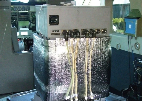
Equipment and a methodology have now been developed for airborne gravity measurements aboard AN-30-type aircraft using inertia-free vibrating-string gravimeters with an error of 0.7–0.8 mGal, meeting the requirements for gravity surveys at 1:200000.

In recent years, airborne gravity investigations in our country have been concentrated primarily at GNPP Aerogeofizika. It is currently the only Russian company with experience of production-scale surveys at 1:200000.

As an example, Figure 2 presents a Bouguer gravity anomaly map derived from an airborne gravity survey in the northern Arkhangelsk Region over 14000 km2 within four topographic map sheets at 1:200000. Survey productivity was approximately 10000 km2 per month. An equivalent map compiled from ground and marine gravity surveys at 1:200000 is shown alongside for comparison. All features of the gravity field over land (the central and southern parts of the area) agree between the maps. The substantial difference in the northern part, over the White Sea, reflects the absence of a reasonably complete and regular network of marine gravity stations there. The error of the airborne gravity map, assessed against high-accuracy (0.25 mGal) ground data at more than one thousand points, is 0.76 mGal. The map has a spatial resolution of 5–6 km.

These materials convincingly demonstrate the suitability of airborne gravimetry for medium-scale (1:200000) gravity field mapping over extensive inaccessible areas.

The Earth’s gravity field is also successfully investigated using satellite data. This raises the question of distinguishing the applications of airborne surveying and satellite gravimetry, particularly satellite altimetry over water. Satellite altimetry investigations have been conducted for approximately 30 years. Two projects are currently operating: the American TOPEX/POSEIDON and the European ERS, with approximately similar accuracy characteristics.

The primary altimetry results are mean satellite heights above the water surface, recorded at approximately 1 Hz over a footprint elongated 6–7 km along the flight path and approximately 1 km wide. These measurements are used to determine geoid heights and gravity field disturbances.

Several catalogues of the Earth’s gravity field now exist in which gravity values over marine areas are obtained from altimetry data (land anomalies are calculated from small-scale ground surveys and observations of artificial Earth satellite orbit perturbations). One of the most complete is the catalogue by Sandwell D. and Smith W., version 9.2 [6].

A gravity anomaly map compiled from this catalogue for the airborne survey area in the Arkhangelsk Region is also shown in Fig. 2. Its error is 4.4 mGal. Other researchers have obtained similar estimates by comparing altimetry and gravity data in different parts of the World Ocean [1,5]. This supports the conclusion that, in detail and accuracy, models of the Earth’s anomalous gravity field derived from satellite altimetry correspond to gravity surveys at 1:1 000 000 and smaller scales. Several fundamental characteristics of the method preclude expectations of substantial improvement in these parameters in the foreseeable future. Satellite gravimetry is therefore not an alternative to airborne surveying for medium-scale work.

In addition to fixed-wing measurements, GNPP Aerogeofizika conducts experimental airborne gravity surveys using helicopters, whose substantially lower flight speed provides greater survey detail. The results demonstrate the feasibility of airborne gravity surveying with an error of 0.3–0.5 mGal and a spatial resolution of 2–3 km. These parameters correspond to large-scale (1:100000–1:50000) gravity surveys in inaccessible areas.

Abroad (in the USA, Canada, and Australia), research is conducted both by public institutions (Lamont-Doherty Earth Observatory , US National Science Foundation , and others) and by major commercial companies (Carson Services, Edcon Aero Surveys, Sander Geophysics, Fugro LCT). Their surveys have the same accuracy parameters as those of GNPP Aerogeofizika.

The list of online communications and publications on airborne gravimetry now contains several hundred entries. This indicates that widespread practical adoption of the new airborne method of measuring gravity has begun in geophysical investigations.

Let us consider the role of airborne gravimetry in investigating the Earth’s gravity field. From the full range of possible gravity field heterogeneities, we first select the class of anomalies whose parameters make them potential targets for airborne gravity measurements, and then assess the distortions inevitable when measuring gravity aboard a moving aircraft. Hereafter, Faye anomalies are conventional anomalies after application of the free-air correction. Bouguer anomalies result from subtracting the attraction, at the measurement point, of all topographic masses between the geoid and the physical land surface, and adding the mass deficit between the seabed and sea level over water.

As a first approximation, any individual anomaly crossed by a survey line can be characterized by just two parameters: amplitude and horizontal extent (conventionally, its extent can be taken as the width of the zone within which the anomaly exceeds 30% of its maximum). It is represented by a point on a graph with these quantities as axes. Identifying anomalies potentially recordable by airborne surveying thus reduces to outlining the corresponding set of points.

The intensity and horizontal dimensions of gravity anomalies are not entirely independent parameters. Unlike magnetization, rock density contrast can vary only within a very limited range. Consequently, a substantial excess mass in a geological body, which determines the intensity of the corresponding gravity anomaly, can arise only from large geometric dimensions. Local anomalies of very large amplitude therefore do not occur in the gravity field.

Accordingly, we first attempted to identify on the coordinate plane the set of points corresponding to anomalies that may be encountered in the air. This was achieved by modelling plausible physiographic and geological situations. Clearly, anomalies with horizontal dimensions ranging from a few kilometres to a few tens of kilometres are of greatest interest. Smaller field structures are targets for detailed ground gravity surveys, whereas the ability to map larger anomalies by airborne surveying is beyond doubt.

The distance between the survey level and potential density heterogeneities is a key modelling parameter. To minimize disturbing accelerations, airborne gravity measurements are made at constant barometric altitude without following the terrain. Flight altitude is therefore generally determined by the terrain within the survey area. Over the targets of greatest interest for hydrocarbon exploration—extensive plains in the Asian part of the country with relatively subdued relief and the marine shelf—flights are usually conducted a few hundred metres above mean ground elevation or sea level.

The modelling results are shown in Figures 3A and 3B (with logarithmic horizontal axes). Curves 1 and 2 provide upper bounds for the set of points corresponding to most possible Faye anomalies at a survey level of 300–400 m above land (excluding mountainous regions) and the shelf. In other words, the anomalies most commonly encountered over land and sea occupy the areas below the respective curves. We shall call these the domains of existence of free-air anomalies.

Let us assess what proportion of these anomalies can be recorded in flight. Measurements aboard an aircraft, as with any survey on a moving platform, are subject to two factors that fundamentally prevent detection of every feature of the true gravity field: limited accuracy and limited detail. The latter results from the need for low-pass filtering during processing to suppress short-period disturbing accelerations. In airborne gravity surveys, instantaneous readings from inertia-free vibrating-string gravimeters are processed with a symmetric filter, such as a cosine Hamming filter. This procedure causes amplitude distortions of the field but no phase distortions.

We shall regard an anomaly identified in a survey as reliable if its amplitude after filtering exceeds twice the measurement error [2]. Curves 3–5 in Fig. 3A show the minimum anomaly amplitudes satisfying this criterion for three different filtering intervals and a survey error of 0.75 mGal. Curves 3–6 in Fig. 3B correspond to filtering over an 8 km interval at different error levels.

Each such line, together with curve 1 or 2, bounds an area on the coordinate plane. All anomalies within it may occur during a survey and, if they do, their presence will be reliably established for the corresponding measurement accuracy and filtering interval. These areas may be called the operational domains of airborne gravimetry.

Currently, for An-30-type aircraft, the lower bound of the operational domain of airborne gravimetry is the curve with parameters of 8 km and 0.75 mGal. The curve with parameters of 4 km and 0.5 mGal corresponds to surveys using a Mi-8 helicopter. Expansion of the operational domain to the curve with parameters of 2 km and 0.25 mGal is a realistic future prospect. For clarity, all three domains, numbered 1, 2, and 3 respectively, are shown in Fig. 3C.

Thus, in fixed-wing surveys, small anomalies with horizontal dimensions of 1–2 km will be recorded only if their amplitudes exceed 6–10 mGal. Local anomalies extending 3–5 km are identified if their intensity exceeds 2–4 mGal. For regional anomalies larger than 7–8 km, amplitudes of 1.5–2 mGal are sufficient. In helicopter surveys, kilometre-scale anomalies are recorded if their amplitudes exceed 2–3 mGal, while from 3–4 km upwards, amplitudes of 1–1.5 mGal suffice for detection.

For a specific geological section, the geological information content of airborne gravimetry can be assessed, giving its operational domains “geological content.” For example, at a mean basement depth of 1 km, anomalies from individual basement blocks 3–4 km across fall within operational domain 1 (Fig. 3С) if their relative uplift or subsidence is 300–400 m. Such structures can therefore be identified by fixed-wing airborne gravity surveys. If basement depths vary over a range of 100–200 m, the corresponding gravity anomalies fall within operational domain 2 and require helicopter measurements for detection.

Let us now assess the possible magnitude of gravity anomaly distortions caused by filtering in airborne surveys. Since Faye anomalies reflect both topographic and geological heterogeneities, the following evident identity can be written:

∆g= ∆g* + (∆g_р — ∆g_р*)+ (∆g_г — ∆g_г*)

where ∆g* is the averaged (filtered) value of ∆g, and the subscripts р and г denote anomaly components caused by terrain irregularities and geological factors, respectively.

Thus, field distortion at any point in an airborne survey consists of two parts, one of which—the first parenthetical term—can be calculated and accounted for. Topographic masses, having a large density contrast relative to the surrounding medium and being closest to the survey level, generally produce the highest-frequency component of the measured gravity field. The first parenthetical term therefore describes a substantial part of the distortion, and accounting for it brings the measured results closer to the true Faye anomaly values.

This is precisely the procedure used in the so-called indirect interpolation of Faye anomalies [4] that we employ to construct the corresponding maps. Its essence is that line data, after accounting for the attraction of topographic masses (filtered Bouguer anomalies), are interpolated onto a regular grid, at whose nodes unsmoothed terrain corrections are then restored.

Let us estimate the second parenthetical term, which represents irreducible gravity field distortions caused by data filtering. By modelling possible geological situations with realistic rock density contrasts, a domain of existence analogous to those described above was constructed, this time for Bouguer anomalies (Fig. 3D, curve 1). Curves 2–4 on the same plot show the maximum possible gravity anomaly distortions as a function of horizontal dimensions for three options for smoothing the original data with a Hamming filter.

When filtering over an 8 km interval, distortions of anomalies extending less than 3–4 km along the survey line may exceed twice the actual airborne survey error. Distortions of anomalies 6–12 km across are comparable to the measurement error. Larger field structures are recorded with practically no distortion. In reality, distortions are usually smaller, since these estimates apply to intense anomalies, which are relatively uncommon.

REFERENCES

1. Ermakov B. V. et al. “Equatorial Shear Zone: Integrated Analysis of a Unique Geological and Geophysical Setting.” RFBR Grant No. 08-05-64927, Moscow, 1999.

2. Instructions for Gravity Prospecting. Moscow, 1980.

3. Lozinskaya A. M., Mogilevsky V. E., Popokov S. G., Fedynsky V. V., Yashayaev I. L. “Gravity Measurements aboard an Aircraft.” Applied Geophysics, Issue 82, Moscow, 1976.

4. Ogorodova L. V., Shimbirev B. P., Yuzefovich A. P. Gravimetry. Moscow, 1978.

5. McAddo D.C., Childers V.A., Laxon S. “ERS satelite gravity and airborne gravity over the Atlantic Ocean : a comparison” Earth System Monitor Vol. 9, No 1, 1998.

6. Sandwell D.T. and Smith W.H.F. “Marine Gravity from Geosat and ERS1 Satelite Altimetry” J. Geoph. Res. V 102 no B5, pp 10039-10054, 1997